Optimal Sequence Alignment Using Dynamic Programming

The Needleman-Wunsch algorithm is the one of the most popular algorithms for global sequence alignment. Its variant, Smith-Waterman algorithm is used for local alignment.

Needleman-Wunsch

Creating the Matrix and Utility Methods

The first step of the Needleman-Wunsch algorithm is to set up the alignment matrix. We add one extra row and column in case the alignment starts with a gap.

m = len(seq1)
n = len(seq2)
mat = [[0 for _ in range(m+1)] for _ in range(n+1)]

We also define a utility method for calculating the score based on the given scoring matrix.

BLOSUM62 = {
    ("W", "F"): 1, ("L", "R"): -2, ("S", "P"): -1, ("V", "T"): 0,
    ("Q", "Q"): 5, ("N", "A"): -2, ("Z", "Y"): -2, ("W", "R"): -3,
    ("Q", "A"): -1, ("S", "D"): 0, ("H", "H"): 8, ("S", "H"): -1,
    ("H", "D"): -1, ("L", "N"): -3, ("W", "A"): -3, ("Y", "M"): -1,
    ("G", "R"): -2, ("Y", "I"): -1, ("Y", "E"): -2, ("B", "Y"): -3,
    ("Y", "A"): -2, ("V", "D"): -3, ("B", "S"): 0, ("Y", "Y"): 7,
    ("G", "N"): 0, ("E", "C"): -4, ("Y", "Q"): -1, ("Z", "Z"): 4,
    ("V", "A"): 0, ("C", "C"): 9, ("M", "R"): -1, ("V", "E"): -2,
    ("T", "N"): 0, ("P", "P"): 7, ("V", "I"): 3, ("V", "S"): -2,
    ("Z", "P"): -1, ("V", "M"): 1, ("T", "F"): -2, ("V", "Q"): -2,
    ("K", "K"): 5, ("P", "D"): -1, ("I", "H"): -3, ("I", "D"): -3,
    ("T", "R"): -1, ("P", "L"): -3, ("K", "G"): -2, ("M", "N"): -2,
    ("P", "H"): -2, ("F", "Q"): -3, ("Z", "G"): -2, ("X", "L"): -1,
    ("T", "M"): -1, ("Z", "C"): -3, ("X", "H"): -1, ("D", "R"): -2,
    ("B", "W"): -4, ("X", "D"): -1, ("Z", "K"): 1, ("F", "A"): -2,
    ("Z", "W"): -3, ("F", "E"): -3, ("D", "N"): 1, ("B", "K"): 0,
    ("X", "X"): -1, ("F", "I"): 0, ("B", "G"): -1, ("X", "T"): 0,
    ("F", "M"): 0, ("B", "C"): -3, ("Z", "I"): -3, ("Z", "V"): -2,
    ("S", "S"): 4, ("L", "Q"): -2, ("W", "E"): -3, ("Q", "R"): 1,
    ("N", "N"): 6, ("W", "M"): -1, ("Q", "C"): -3, ("W", "I"): -3,
    ("S", "C"): -1, ("L", "A"): -1, ("S", "G"): 0, ("L", "E"): -3,
    ("W", "Q"): -2, ("H", "G"): -2, ("S", "K"): 0, ("Q", "N"): 0,
    ("N", "R"): 0, ("H", "C"): -3, ("Y", "N"): -2, ("G", "Q"): -2,
    ("Y", "F"): 3, ("C", "A"): 0, ("V", "L"): 1, ("G", "E"): -2,
    ("G", "A"): 0, ("K", "R"): 2, ("E", "D"): 2, ("Y", "R"): -2,
    ("M", "Q"): 0, ("T", "I"): -1, ("C", "D"): -3, ("V", "F"): -1,
    ("T", "A"): 0, ("T", "P"): -1, ("B", "P"): -2, ("T", "E"): -1,
    ("V", "N"): -3, ("P", "G"): -2, ("M", "A"): -1, ("K", "H"): -1,
    ("V", "R"): -3, ("P", "C"): -3, ("M", "E"): -2, ("K", "L"): -2,
    ("V", "V"): 4, ("M", "I"): 1, ("T", "Q"): -1, ("I", "G"): -4,
    ("P", "K"): -1, ("M", "M"): 5, ("K", "D"): -1, ("I", "C"): -1,
    ("Z", "D"): 1, ("F", "R"): -3, ("X", "K"): -1, ("Q", "D"): 0,
    ("X", "G"): -1, ("Z", "L"): -3, ("X", "C"): -2, ("Z", "H"): 0,
    ("B", "L"): -4, ("B", "H"): 0, ("F", "F"): 6, ("X", "W"): -2,
    ("B", "D"): 4, ("D", "A"): -2, ("S", "L"): -2, ("X", "S"): 0,
    ("F", "N"): -3, ("S", "R"): -1, ("W", "D"): -4, ("V", "Y"): -1,
    ("W", "L"): -2, ("H", "R"): 0, ("W", "H"): -2, ("H", "N"): 1,
    ("W", "T"): -2, ("T", "T"): 5, ("S", "F"): -2, ("W", "P"): -4,
    ("L", "D"): -4, ("B", "I"): -3, ("L", "H"): -3, ("S", "N"): 1,
    ("B", "T"): -1, ("L", "L"): 4, ("Y", "K"): -2, ("E", "Q"): 2,
    ("Y", "G"): -3, ("Z", "S"): 0, ("Y", "C"): -2, ("G", "D"): -1,
    ("B", "V"): -3, ("E", "A"): -1, ("Y", "W"): 2, ("E", "E"): 5,
    ("Y", "S"): -2, ("C", "N"): -3, ("V", "C"): -1, ("T", "H"): -2,
    ("P", "R"): -2, ("V", "G"): -3, ("T", "L"): -1, ("V", "K"): -2,
    ("K", "Q"): 1, ("R", "A"): -1, ("I", "R"): -3, ("T", "D"): -1,
    ("P", "F"): -4, ("I", "N"): -3, ("K", "I"): -3, ("M", "D"): -3,
    ("V", "W"): -3, ("W", "W"): 11, ("M", "H"): -2, ("P", "N"): -2,
    ("K", "A"): -1, ("M", "L"): 2, ("K", "E"): 1, ("Z", "E"): 4,
    ("X", "N"): -1, ("Z", "A"): -1, ("Z", "M"): -1, ("X", "F"): -1,
    ("K", "C"): -3, ("B", "Q"): 0, ("X", "B"): -1, ("B", "M"): -3,
    ("F", "C"): -2, ("Z", "Q"): 3, ("X", "Z"): -1, ("F", "G"): -3,
    ("B", "E"): 1, ("X", "V"): -1, ("F", "K"): -3, ("B", "A"): -2,
    ("X", "R"): -1, ("D", "D"): 6, ("W", "G"): -2, ("Z", "F"): -3,
    ("S", "Q"): 0, ("W", "C"): -2, ("W", "K"): -3, ("H", "Q"): 0,
    ("L", "C"): -1, ("W", "N"): -4, ("S", "A"): 1, ("L", "G"): -4,
    ("W", "S"): -3, ("S", "E"): 0, ("H", "E"): 0, ("S", "I"): -2,
    ("H", "A"): -2, ("S", "M"): -1, ("Y", "L"): -1, ("Y", "H"): 2,
    ("Y", "D"): -3, ("E", "R"): 0, ("X", "P"): -2, ("G", "G"): 6,
    ("G", "C"): -3, ("E", "N"): 0, ("Y", "T"): -2, ("Y", "P"): -3,
    ("T", "K"): -1, ("A", "A"): 4, ("P", "Q"): -1, ("T", "C"): -1,
    ("V", "H"): -3, ("T", "G"): -2, ("I", "Q"): -3, ("Z", "T"): -1,
    ("C", "R"): -3, ("V", "P"): -2, ("P", "E"): -1, ("M", "C"): -1,
    ("K", "N"): 0, ("I", "I"): 4, ("P", "A"): -1, ("M", "G"): -3,
    ("T", "S"): 1, ("I", "E"): -3, ("P", "M"): -2, ("M", "K"): -1,
    ("I", "A"): -1, ("P", "I"): -3, ("R", "R"): 5, ("X", "M"): -1,
    ("L", "I"): 2, ("X", "I"): -1, ("Z", "B"): 1, ("X", "E"): -1,
    ("Z", "N"): 0, ("X", "A"): 0, ("B", "R"): -1, ("B", "N"): 3,
    ("F", "D"): -3, ("X", "Y"): -1, ("Z", "R"): 0, ("F", "H"): -1,
    ("B", "F"): -3, ("F", "L"): 0, ("X", "Q"): -1, ("B", "B"): 4
}

def score_prot(i, j):
    if (i, j) in BLOSUM62:
        return BLOSUM62[(i, j)]
    else:
        return BLOSUM62[(j, i)]

Populate the First Row and Column of the Matrix

We first populate the first row and column with gap penalty scores.

for i in range(len(seq1) + 1):
		mat[0][i] = gap_penalty * i
for j in range(len(seq2) + 1):
		mat[j][0] = gap_penalty * j

Filling in the Rest of the Matrix

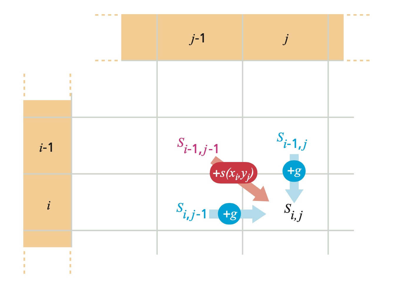
We fill in the rest of the matrix with scores calculated using this formula:

$$
M(i,j)=\max\begin{cases}
M(i-1,j-1)+s(i,j) \
M(i-1,j)+g \
M(i,j-1)+g
\end{cases}
$$

$s(i,j)$ is the score of $i$ aligning with $j$. $M(i,j)$ is the value at location $i,j$ in the Needleman-Wunsch matrix. $g$ is the gap penalty (assuming linear penalty).

The diagonal path from $M(i-1,j-1)$ to $M(i,j)$ indicates a match. A horizontal path or vertical path indicates an indel (insertion or deletion, gap).

for i in range(1, len(seq2) + 1):
		for j in range(1, len(seq1) + 1):
		    # seq2 insertion/seq1 deletion
				score_horizontal = mat[i][j-1] + gap_penalty
		    # seq2 deletion/seq1 insertion
		    score_vertical = mat[i-1][j] + gap_penalty
		    score_diagonal = mat[i-1][j-1] + score_nt(seq1[j-1], seq2[i-1])
		    mat[i][j] = max(score_horizontal, score_vertical, score_diagonal)

The formula used to calculate each individual score ensures that the assigned score is always produced from the highest scoring path. By the principles of dynamic programming, we can combine the optimal solutions of subproblems (local highest-scoring paths) to find the solution to the overall problem (highest-scoring global alignment).

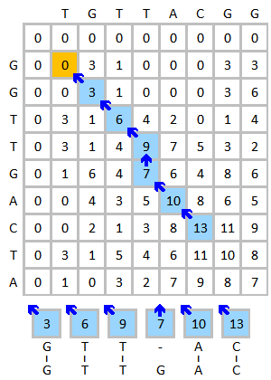
Tracing Back

Since we know that by combining optimal subproblem solutions, we can get the optimal overall solution, we can find the best global alignment by tracing back along the highest-scoring path from the bottom-right corner to the origin.

while i > 0 and j > 0:
		score_current = mat[i][j]
		score_up = mat[i-1][j]
		score_left = mat[i][j-1]
		score_diagonal = mat[i-1][j-1]
		if score_current == score_diagonal + score_nt(seq1[j-1], seq2[i-1]):
		    aligned1 += seq1[j-1]
		    aligned2 += seq2[i-1]
		    i -= 1
		    j -= 1
		elif score_current == score_up + gap_penalty:
		    aligned1 += '-'
		    aligned2 += seq2[i-1]
		    i -= 1
		elif score_current == score_left + gap_penalty:
		    aligned1 += seq1[j-1]
		    aligned2 += '-'
		    j -= 1

In case of leading gaps, we prepend the gaps.

while i > 0:
    aligned1 += '-'
    aligned2 += seq2[i-1]
    i -= 1
    
while j > 0:
    aligned1 += seq1[j-1]
    aligned2 += '-'
    j -= 1

Since we get the result by tracing backwards, the result is reversed. To get the actual result, we simply invert the string.

aligned1, aligned2 = aligned1[::-1], aligned2[::-1]

Time Complexity Analysis

The big-O time complexity of the Needleman-Wunsch algorithm is $O(mn)$ because ultimately we have to go through every element in the matrix. However, by doing some optimization and preprocessing, we can improve the runtime complexity and optimize the constant terms and factors.

Smith-Waterman

Smith-Waterman is a modified version of Needleman-Wunsch algorithm used for local alignment problems. Rather than attempting to align the whole sequence, local alignment algorithms align the most similar (conserved) regions/segments within the sequences to be aligned. Smith-Waterman’s main difference from Needleman-Wunsch is that it uses a slightly different formula to fill in the matrix.

$$
M(i,j)=\max\begin{cases}
M(i-1,j-1)+s(i,j) \
M(i-1,j)+g \
M(i,j-1)+g \
0
\end{cases}
$$

Basically, whenever the score falls below zero, the score is set equal to zero. By doing so, the high-scoring segments can easily stand out from the rest of the matrix.

For the traceback step, we starts from the element with the highest score and stops when we hit zero.

# locate the max
i = 0
j = 0
max_temp = mat[i][j]
for i_temp in range(0, len(seq2)+1):
    for j_temp in range(0, len(seq1)+1):
        if mat[i_temp][j_temp] > max_temp:
            max_temp = mat[i_temp][j_temp]
            i, j = i_temp, j_temp
            
# backtrace to find the alignment
while i > 0 and j > 0 and mat[i][j] != 0:
    score_current = mat[i][j]
    score_up = mat[i-1][j]
    score_left = mat[i][j-1]
    score_diagonal = mat[i-1][j-1]
    if score_current == score_diagonal + score_nt(seq1[j-1], seq2[i-1]):
        aligned1 += seq1[j-1]
        aligned2 += seq2[i-1]
        i -= 1
        j -= 1
    elif score_current == score_up + gap_penalty:
        aligned1 += '-'
        aligned2 += seq2[i-1]
        i -= 1
    elif score_current == score_left + gap_penalty:
        aligned1 += seq1[j-1]
        aligned2 += '-'
        j -= 1
        
while i > 0:
    aligned1 += '-'
    aligned2 += seq2[i-1]
    i -= 1

while j > 0:
    aligned1 += seq1[j-1]
    aligned2 += '-'
    j -= 1
    
aligned1, aligned2 = aligned1[::-1], aligned2[::-1]

EMBOSS - Needle, Water, Stretcher, and Matcher

EMBOSS (European Molecular Biology Open Software Suite) is a set of bioinformatics tools. Its online version is hosted by EMBL-EBI on https://www.ebi.ac.uk/Tools/emboss/

EMBOSS programs < EMBL-EBI

EMBOSS includes Needle and Water, two alignment tools developed using the Needleman-Wunsch and Smith-Waterman, respectively.

To use Needle or Water only, simply go to the website and paste sequence. We can choose the scoring matrix used to align two sequences as well as gap penalties. They use an affine penalty for gap extension, which is also the more widely used gap penalty function. The affine gap penalty increases by a certain amount when a gap is extended. It is implemented by keeping track of three set of scores, as opposed to one set for linear penalty. The score is assigned using the following set of formulas:

$$
M(i,j)=\max\begin{cases}
M(i-1,j-1)+s(i,j) \
I_x(i-1,j-1)+s(i,j) \
I_y(i-1,j-1)+s(i,j)
\end{cases}
$$

$$
I_x(i,j)=\max\begin{cases}
M(i-1,j)+h+g \
I_x(i-1,j)+g
\end{cases}
$$

$$
I_y(i,j)=\max\begin{cases}
M(i,j-1)+h+g \
I_y(i,j-1)+g
\end{cases}
$$

where $h$ is the gap opening penalty and $g$ is the gap extension penalty.

EMBOSS also has a command-line version. The mandatory qualifiers are asequence, bsequence, gapopen, gapextend, and outfile.

needle -asequence=SEQUENCE1 -bsequence=SEQUENCE2 -gapopen=GAP_OPEN_PENALTY -gapextend=GAP_EXTENSION_PENALTY -outfile=OUTPUT

For example, we use the following command to align two sequences named sarsspike.fa and sars2spike.fa with a gap open penalty of 10, gap extension penalty of 0.5, and print the result to stdout.

needle -asequence=sarsspike.fa -bsequence=sars2spike.fa -gapopen=10 -gapextend=0.5 -outfile=stdout

We can also specify the scoring matrix using the qualifier -datafile. The built-in data files are located at .../EMBOSS/data.

Stretcher is a rapid global alignment tool built using optimized Needleman-Wunsch algorithm, and Matcher is a rapid local alignment tool built using optimized Smith-Waterman.

EMBOSS: needle

EMBOSS: water

EMBOSS: stretcher

EMBOSS: matcher

Reference

Pevsner, J. (2016). Bioinformatics and Functional Genomics. Chichester, West Sussex: Wiley Blackwell.

Zvelebil, M. J., & Baum, J. O. (2008). Understanding Bioinformatics. New York: Garland Science/Taylor & Francis Group.

Christopher Burge, David Gifford, and Ernest Fraenkel. 7.91J Foundations of Computational and Systems Biology. Spring 2014. Massachusetts Institute of Technology: MIT OpenCourseWare, https://ocw.mit.edu. License: Creative Commons BY-NC-SA.